3  Remote Sensing Data

Week 3 focused on the processing involved in producing analysis-ready data products from raw images.

3.1 Summary

3.1.1 Satellite Data Acquisition

There are two ways in which satellites collect remotely sensed data.

Table 3.1: Table contrasting whisk and push broom methods. Image Sources: Shippert (n.d.)

	Push Broom	Whisk Broom
Description	A continuous line, covering a large swath over a large study area.	Taking multiple passes over a more localised study area.
Image
Benefits	Efficient over a large scale, covering a wide area in one go.	Higher spatial resolution
Limitations	Lower spatial resolution	Slower than push broom method

3.1.2 Distortions

Various distortions can impact upon the quality, accuracy and reliability of remotely sensed data.

• View angle: refers to variation between the angle of incidence and angle of reflectance
• Topography: refers to the impact elevation has, as flat and sloped areas vary in reflectance.
• Rotation of earth: Earth’s position relative to the sun impacts illumination, impacting passive sensors.

3.1.3 Corrections

Due to natural variability, corrections are used to remove the impacts various factors have on collected images to give a more accurate view of the study area.

3.1.3.1 Geometric Correction

This is used to address the distortions introduced from the satellite viewing angle. This involved the recorded image coordinates being mapped against their ground truth counterparts, with the addition of mathematical transformations to benefit the scale and rotation of the image.

3.1.3.2 Atmospheric Correction

Removing the effects of atmospheric interference on imagery, to improve quality. Interference comes from the scattering of incoming light, and the absorption of that being reflected. Both of which can result in a poor representation of the study area.

See Figure 3.1 as a graphical description.

Figure 3.1: The need for atmospheric corrections. Source: Link

3.1.3.3 Empirical Line Correction

Comparing the reflectance values of a known target, also known as ground truth measurements. Linear regression can be applied to allow the identification of variation between real-world values and those that are remotely monitored.

3.1.3.4 Topographic (Orthorectification) Correction

Correcting for topographic features disrupting the reluctance values, as caused by shadows and slopes. By identifying the Solar Zenith Angle (SZA) and the Viewing Zenith Angle (VZA) the amount of illumination of the target area can be calculated, allowing essential correction to represent the study area.

3.1.3.5 Radiometric Correction

Adjusting the values of imagery to account for variation within the sensitivity of the sensor. Therefore, allowing for a more consistent account of the conditions being monitored within the study area.

3.1.4 Enhancements

Combining several bands of remote-sensing imagery allow for enhancements such as the Normalized Difference Vegetation Index (NDVI) to be created, allowing the identification of vegetation health and abundance. Key additional enhancements can be seen in Table 3.2.

Table 3.2: Table of interesting remote sensing enhancements.

Enhancement	Abbreviation	Definition	Equation
Normalized Difference Vegetation Index	NDVI	The proportion of healthy vegetation.	(NIR - Red) / (NIR + Red)
Normalized Difference Water Index	NDWI	The abundance of water in remote sensing imagery.	(NIR - SWIR) / (NIR + SWIR)
Normalized Difference Snow Index	NDSI	The abundance of snow and ice in remote sensing imagery.	(Green/Red/SWIR - Green/Red/SWIR)
Normalized Difference Moisture Index	NDMI	The abundance of moisture in remote sensing imagery.	(NIR - MIR) / (NIR + MIR)

See Figure 3.2 for a summary of NDVI.

Figure 3.2: NDVI Meme. Source: Link

3.2 Applications

Ilori, Pahlevan, and Knudby (2019)’s research worked to investigate how four atmospheric correction algorithms performed when being applied to Landsat 8 imagery of coastal waters. The four atmospheric correction models were:

• Atmospheric and Radiometric Correction of Satellite Imagery (ARCSI).
• Atmospheric Correction for OLI lite (ACOLITE).
• Landsat 8 Surface Reflectance Climate Data Record (LaSRC).
• Sea-Viewing Wide Field-of-View Sensor Data Analysis System (SeaDAS).

It was found that generic methods of atmospheric correction, such as LaSRC, perform reasonably well over land but have shortcomings when looking at ocean imagery (particularly in the blue bands). Water-specific atmospheric correction methods (SeaDAS and ACOLITE) have much greater reliability and accuracy. The two largest external contributors to errors were identified to be wind speed and solar zenith angle, as can be seen in Table 3.3.

Table 3.3: Table of key errors identified in Ilori, Pahlevan, and Knudby (2019)’s research, and their reasoning.

Responsible factor	Reasoning
Solar Zenith Angle (SZA)	High SZAs lead to reductions in the concentration of light entering the atmosphere.
Wind Speed	Prevlaining wind of high-speed causes waves to impact the surface roughness. This in turn changes the proportion of light being reflected and absorbed by the water.

As these methods are used to plot bathymetric maps, it is essential to address and correct the inherent errors in the imagery. If not, it could lead to ships and other vessels becoming grounded.

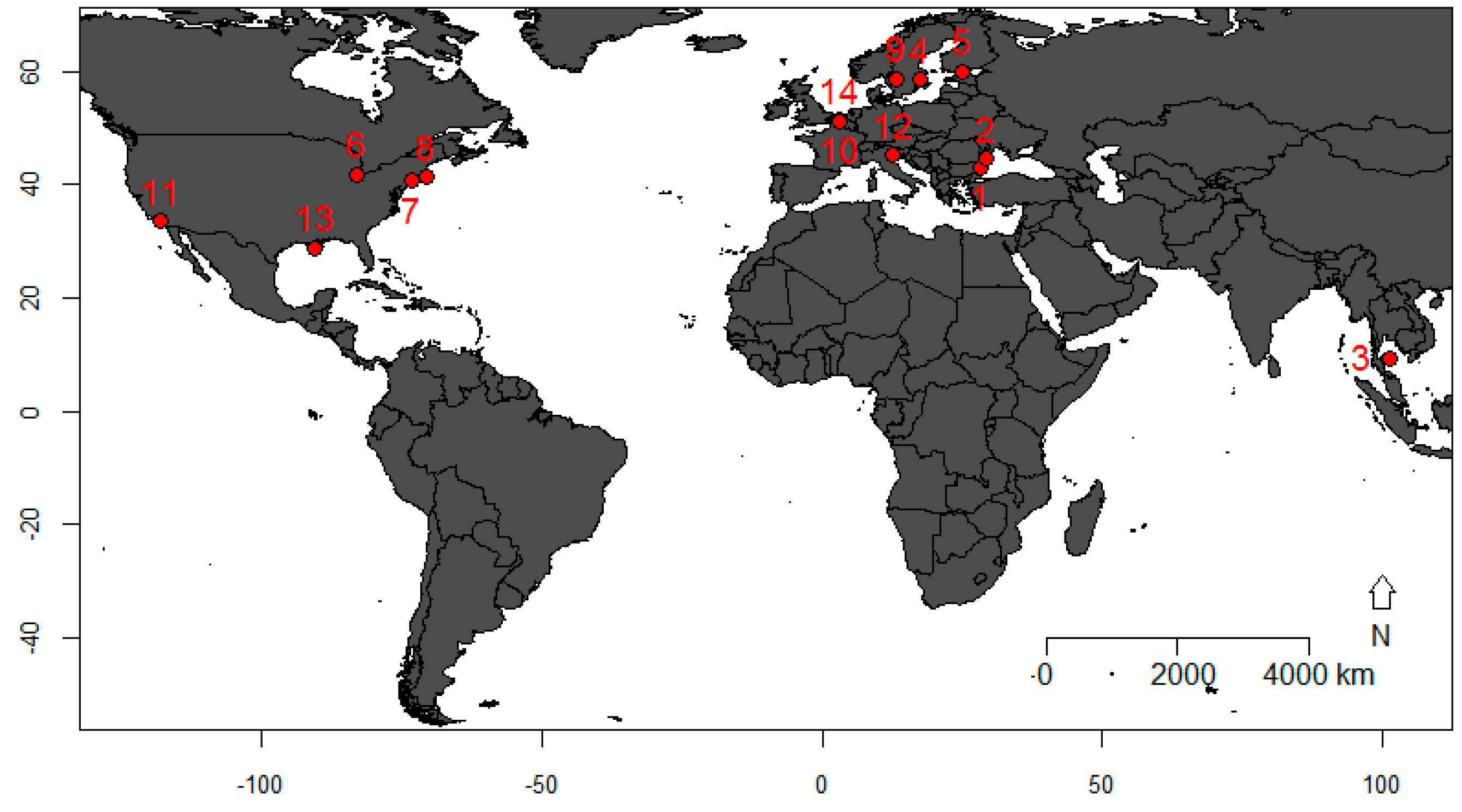
Although Ilori, Pahlevan, and Knudby (2019)‘s work made use of 14 validation sites, they were solely located within the ’global North’, as can be seen in Figure 3.3. This becomes problematic when additional factors may be present in the ‘global South’ that should be considered. For example, Okafor-Yarwood and Adewumi (2020) identified that while developed nations tend to dispose of their waste through landfill, less developed countries can sometimes resort to dumping their waste into their oceans. This is likely to have a large impact on the remote sensing capabilities specifically when trying to map bathymetry.

Figure 3.3: Mapped location of validation sites for Ilori, Pahlevan, and Knudby (2019)’s research.

3.3 Reflection

Correcting remotely sensed data is essential because of the various sources of noise and error that are introduced impacting the quality of the images. As these atmospheric conditions and geometric distortions (causing the error) are not consistent temporally or spatially they must be accurate and reliably corrected to allow for incorrect interpretations and decisions to be avoided.

Wider Applications: In past research, I have had to account for climatological factors when analysing urban air quality, as changes in humidity and wind speed have been found to likely cause changes in airborne pollution concentration. I imagine this will still be the case for remotely sensed data and would provide another step in the methodological process before a final output can be produced. I wonder if any existing libraries can implement remotely sensed pollution data with remotely sensed weather data to provide a standardised and reproducible unit of airborne pollutants. This would be of great benefit to academics and policy advisors when examining urban air pollution mitigation strategies.

Ilori, Christopher O., Nima Pahlevan, and Anders Knudby. 2019. “Analyzing Performances of Different Atmospheric Correction Techniques for Landsat 8: Application for Coastal Remote Sensing.” Remote Sensing 11 (4): 469. https://doi.org/10.3390/rs11040469.

Okafor-Yarwood, Ifesinachi, and Ibukun Jacob Adewumi. 2020. “Toxic Waste Dumping in the Global South as a Form of Environmental Racism: Evidence from the Gulf of Guinea.” African Studies 79 (3): 285–304. https://doi.org/10.1080/00020184.2020.1827947.

Shippert, Peg. n.d. “Push Broom and Whisk Broom Sensors.” L3Harris Geospatial. https://www.l3harrisgeospatial.com/Support/Self-Help-Tools/Help-Articles/Help-Articles-Detail/ArtMID/10220/ArticleID/16262/Push-Broom-and-Whisk-Broom-Sensors. Accessed February 10, 2023.